How Fine-Tuning Warps the Hidden Geometry of Transformers

A transformer is trained to predict tokens, but in the process it learns something richer than a next-token probability distribution. It learns a geometry over tokens and contexts. Hidden states become points in a high-dimensional space, encoding semantic, syntactic, and task-specific information as directions, distances, subspaces, and spectra.

This geometry matters because downstream behavior is often decided by simple operations on these representations, such as linear heads, cosine similarity, nearest-neighbor retrieval, or clustering. If the representation space collapses into a narrow cone, cosine similarity becomes less informative. If fine-tuning concentrates label information in a few principal directions, removing those directions can destroy performance. If LoRA introduces new singular directions, those directions can explain both adaptation and forgetting.

This post gives a compact geometric view of pre-training and fine-tuning, and briefly covers scalable validation.

To make the discussion concrete, I include a small case study comparing distilbert-base-uncased with distilbert-base-uncased-finetuned-sst-2-english on GLUE/SST-2. You can reproduce this experiment and generate the visualizations using the code in the accompanying GitHub repository.

Transformer representations have geometry

Let $\mathcal V$ be a vocabulary and let $d$ be the hidden dimension. The input embedding matrix is

\[E_{\mathrm{in}} \in \mathbb{R}^{|\mathcal V|\times d},\]

so each token index is mapped to a vector in $\mathbb{R}^d$. For a sequence of length $T$, the hidden states at layer $\ell$ are

\[H^{(\ell)} \in \mathbb{R}^{T\times d}.\]

A self-attention head computes

\[\operatorname{Attention}(Q,K,V_{\mathrm{val}}) = \operatorname{softmax}\left(\frac{QK^\top}{\sqrt{d_k}}\right)V_{\mathrm{val}},\]

where $Q$, $K$, and $V_{\mathrm{val}}$ are query, key, and value projections of the current hidden states.

The model also has an output unembedding or language-model head

\[U \in \mathbb{R}^{|\mathcal V|\times d},\]

whose rows act as token classifiers. Given a hidden state $h$, the logit for token $v$ is typically

\[z_v(h)=u_v^\top h+b_v.\]

Some architectures tie $U$ and $E_{\mathrm{in}}$; others keep them separate.

There are two related geometries worth separating:

1. Activation geometry, which is the point cloud formed by hidden states $h_i$ across tokens, positions, layers, and contexts.
2. Weight geometry, or the geometry of learned matrices such as $E_{\mathrm{in}}$, $U$, attention projections, MLP weights, and low-rank adaptation matrices.

Fine-tuning changes both. Full fine-tuning moves all weights, while PEFT methods such as LoRA move only a small number of parameters, making the resulting geometric deformation easier to inspect.

Isotropy and anisotropy

A basic geometric question is whether a representation uses its dimensions evenly.

Given centered hidden states $X\in\mathbb{R}^{N\times d}$, with rows

\[x_i=h_i-\bar h,\]

the empirical covariance is

\[\widehat{\Sigma} = \frac{1}{N-1}X^\top X.\]

The representation is approximately isotropic when

\[\widehat{\Sigma}\approx \sigma^2 I,\]

meaning variance is spread roughly evenly across directions. Equivalently, no small set of principal components dominates the representation.

If $\lambda_1,\ldots,\lambda_d$ are the covariance eigenvalues, a useful summary statistic is the participation-ratio effective rank

\[r_{\mathrm{eff}} = \frac{\left(\sum_i \lambda_i\right)^2}{\sum_i \lambda_i^2}.\]

This quantity is scale-invariant. It equals $d$ when all eigenvalues are equal and approaches $1$ when one direction carries almost all variance.

Transformer representations are often anisotropic, meaning that hidden states can share a large common component, occupy a narrow cone, or have a covariance spectrum dominated by a few directions. These are related but not identical phenomena. A large mean vector affects raw cosine similarity; a concentrated covariance spectrum affects effective rank and explained variance. A representation can look good under one diagnostic and degenerate under another.

This phenomenon of anisotropy in transformer representations is referred to as representation degeneration and has been observed in contextual word representations and language generation models^{[5], [6], [7]}. Similar effects have also been reported outside natural language text, including in protein language models, suggesting that anisotropy is a broader interaction among architecture, data distribution, objective, normalization, and optimization^[8].

A common symptom is high average cosine similarity between unrelated hidden states. If

\[h_i = m+\varepsilon_i\]

and the common component $m$ is large relative to the variation $\varepsilon_i$, then many pairwise cosines become artificially high. This makes angular distance less useful for semantic discrimination.

However, it’s important to note that low average cosine is not evidence of isotropy. A simple counterexample makes this clear. Suppose

\[h_i = y_i v, \qquad y_i\in\{-1,+1\},\]

with roughly balanced signs. The covariance is rank one, so the representation is maximally anisotropic in the sense that all variation lies along the single direction $v$, and $r_{\mathrm{eff}}=1$. But the average pairwise cosine is close to zero, because pairs with the same sign contribute $+1$, pairs with opposite signs contribute $-1$, and the two effects mostly cancel. If the signs are exactly balanced, the average over distinct pairs is $-1/(N-1)$, essentially zero for large $N$.

Why anisotropy can arise

One mechanism comes directly from the softmax objective.

For an autoregressive language model,

\[p_\theta(v\mid c) = \frac{\exp(u_v^\top h_c+b_v)}{\sum_{w\in\mathcal V}\exp(u_w^\top h_c+b_w)},\]

where $h_c$ is the hidden state for context $c$. For a single training example with target token $y$, the cross-entropy gradient with respect to output vector $u_v$ is

\[\nabla_{u_v}\bigl[-\log p_\theta(y\mid c)\bigr] = \left(p_\theta(v\mid c)-\mathbf 1\{v=y\}\right)h_c.\]

For a rare token $v$, most contexts are negative examples, in which $v\neq y$. Gradient descent therefore repeatedly updates $u_v$ in directions that reduce its logit on the bulk of hidden states.

Gao et al. describe a related degeneration mechanism^[7]. Suppose that there exists a direction $a$ such that

\[h_c^\top a < 0\]

for all relevant hidden states $h_c$. Then moving a rare token’s output embedding in the $a$ direction lowers that token’s logit across those contexts. A separating-hyperplane argument can supply such a direction when the origin lies outside the convex hull of the hidden-state cloud.

This helps explain why rare-token output embeddings can acquire common directions under softmax training. If input embeddings and output unembeddings are tied, this output-side pressure can also leak into the input embedding geometry.

This is not the only source of anisotropy, but it is an important example showing that degeneration can be a natural byproduct of the optimization process rather than a mere numerical accident.

Fine-tuning reorganizes geometry

Fine-tuning should not be understood as simply repairing pre-training anisotropy. It often reorganizes the representation space around the downstream objective.

In full fine-tuning, the model is initialized from pre-trained weights $\theta_{\mathrm{pre}}$, and all parameters are updated on a downstream dataset $\mathcal D_{\mathrm{FT}}$ by the rule

\[\theta_{t+1} = \theta_t - \eta \nabla_\theta \mathcal L_{\mathrm{FT}}(\theta_t;\mathcal D_{\mathrm{FT}}).\]

At the activation level, fine-tuning changes the covariance of hidden states. For centered samples from layer $\ell$,

\[X^{(\ell)}\in\mathbb{R}^{N\times d},\]

define

\[C^{(\ell)} = \frac{1}{N-1}(X^{(\ell)})^\top X^{(\ell)}.\]

The eigenvalues of $C^{(\ell)}$ describe how concentrated the representation is. The eigenvectors describe where that variance lies.

Before fine-tuning, leading principal components may encode broad or nuisance statistics such as token frequency, punctuation, sentence length, and so on. This helps explain why post-processing methods such as All-but-the-Top, which center embeddings and remove leading principal components, can improve some static embedding and similarity benchmarks^[9].

After fine-tuning, however, dominant directions can become task-relevant. In BERT-like models, fine-tuning may concentrate information useful for natural language inference, semantic textual similarity, or classification into high-variance directions^[3]. The representation may become less isotropic while becoming better for the task.

This provides evidence that removing top principal components is not automatically a cleanup step. If the top components encode nuisance structure, removing them can help, but if they encode label-relevant information, removing them can destroy performance.

A task-aware ablation is better. If $V_k=[v_1,\ldots,v_k]$ contains the top $k$ principal directions of the centered representation, test the intervention

\[h \mapsto \bar h + (I - V_kV_k^\top)(h-\bar h)\]

on the downstream metric, and also test removing low-variance directions. Then, report geometry and task performance together. Isotropy alone is not the objective.

Case study of fine-tuning on DistilBERT’s geometry

The claim above is easy to state but easy to misuse. So let us look at a small diagnostic experiment.

Experimental setup

I compared two public checkpoints:

• distilbert-base-uncased, the pre-trained DistilBERT backbone^[15];
• distilbert-base-uncased-finetuned-sst-2-english, the same architecture fine-tuned for SST-2 sentiment classification.

The evaluation set was the full GLUE/SST-2 validation split, $N=872$ examples^{[16], [17]}. The script did not train either model; rather, it extracted the $[\mathrm{CLS}]$ hidden state at every hidden-state index, which is the embedding output plus the six DistilBERT transformer layers.

For each layer, it computed:

• mean norm $|\bar h|_2$;
• average raw pairwise cosine;
• average centered pairwise cosine;
• covariance eigenvalue spectrum;
• participation-ratio effective rank;
• top-$k$ explained variance;
• pre-trained/fine-tuned PCA subspace overlap;
• task accuracy after ablating principal components from the fine-tuned final-layer $[\mathrm{CLS}]$ states.

The embedding-layer $[\mathrm{CLS}]$ vector is constant across examples in this architecture, so its covariance is zero.

Summary metrics

The final-layer $[\mathrm{CLS}]$ geometry changed sharply after fine-tuning.

Final-layer state	SST-2 accuracy	$|\bar h|_2$	$\operatorname{tr}(\widehat\Sigma)$	Effective rank	Top-1 variance	Top-10 variance	Raw avg. cosine	Centered avg. cosine
Pre-trained backbone	—	11.77	12.58	25.82	13.8%	48.4%	0.917	0.0002
Fine-tuned classifier	0.911	7.59	196.24	1.62	78.3%	90.3%	0.230	0.0016

The pre-trained backbone has no SST-2 classification head, so I do not report a task accuracy for it. The fine-tuned checkpoint reaches $91.1\%$ accuracy on these 872 validation examples.

Raw average cosine drops from $0.917$ to $0.230$, which by itself might suggest that the fine-tuned representation is less anisotropic. But the covariance spectrum says the opposite, as the final fine-tuned $[\mathrm{CLS}]$ states are much more spectrally concentrated. The top principal component alone explains $78.3\%$ of the variance, and the top ten explain $90.3\%$. The effective rank falls from $25.82$ to $1.62$ out of $768$ dimensions.

This is not surprising. A representation can have near-zero average centered cosine while being almost one-dimensional, as long as examples are distributed on both sides of the dominant axis. For a sentiment classifier, that is a plausible geometry, as positive and negative examples may separate along a high-variance direction, causing pairwise cosine contributions to cancel in the average. This demonstrates concretely why relying solely on average cosine to measure anisotropy can be misleading.

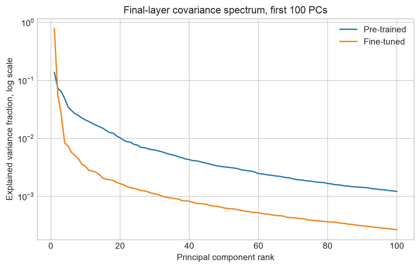
Figure 1. Covariance spectra before and after fine-tuning. Eigenvalues are normalized by total variance. A steeper curve means variance is more concentrated in a small number of directions.

The subspace-overlap diagnostic reinforces this finding. For top-$k$ PCA bases $A$ and $B$, I measured

\[\frac{\|A^\top B\|_F^2}{k}.\]

This equals $1$ for identical $k$-dimensional subspaces and decreases as the subspaces diverge. Ignoring the degenerate embedding layer, the top-10 pre-trained/fine-tuned overlap was about $0.69$ after the first transformer layer, $0.49$ after the fourth, and $0.20$ in the final layer. The top-50 overlap in the final layer was $0.35$. Fine-tuning therefore did not merely rescale the old leading directions; in fact, it substantially reorganized the principal subspaces in later layers.

Principal-component ablation

The decisive question is whether the new dominant directions are useful or harmful.

To test this, I modified the fine-tuned final-layer $[\mathrm{CLS}]$ states by removing principal components and then passed the modified states through the frozen DistilBERT classification head via the intervention

\[h \mapsto \bar h + (I - V_kV_k^\top)(h-\bar h).\]

This intervention was applied only at the final representation, without rerunning the transformer. It tests how much the trained classifier depends on particular representation directions.

Intervention on fine-tuned final $[\mathrm{CLS}]$	SST-2 accuracy
No ablation	0.911
Remove top 1 PC	0.513
Remove top 10 PCs	0.509
Remove top 100 PCs	0.509
Remove bottom 1 PC	0.911
Remove bottom 100 PCs	0.911

Removing the top principal component alone drops accuracy from $91.1\%$ to roughly chance. Removing additional top components does not substantially worsen it, because the main decision-relevant direction has already been removed. By contrast, removing as many as 100 bottom principal components leaves accuracy unchanged.

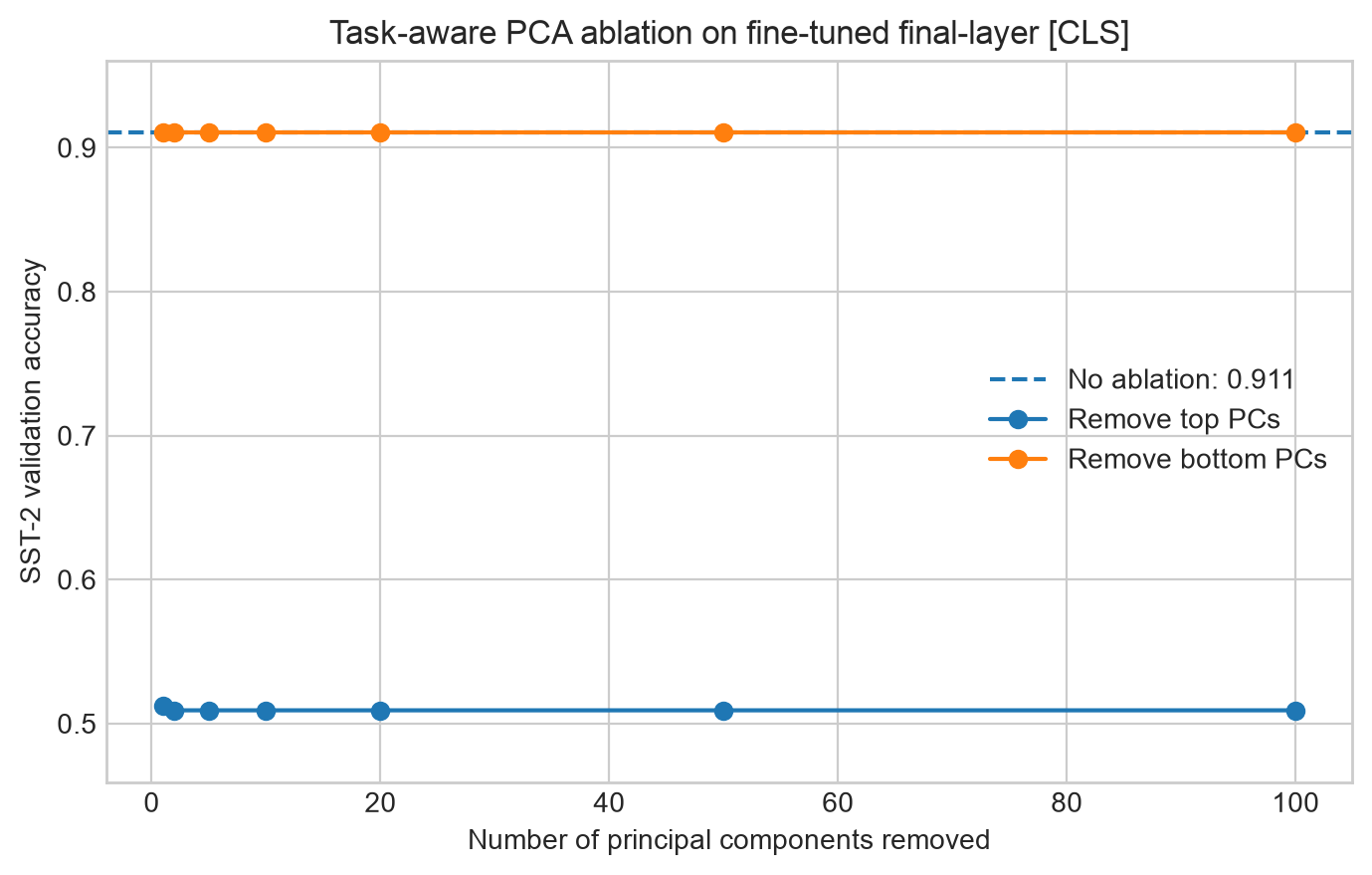
Figure 2. Task performance after principal-component ablation. Removing the top principal components tests whether high-variance directions encode nuisance structure or task-relevant information. Removing bottom components serves as a control.

This is the main lesson of the case study. The final fine-tuned representation is highly anisotropic in the centered covariance sense, but that anisotropy is not merely collapse. At least for the SST-2 classifier, the dominant direction is task-critical.

There is one methodological caveat. In this small blog experiment, PCA directions were estimated on the same validation activations that were later ablated. The labels were not used to fit the PCs, but a stricter benchmarking evaluation should fit PCA directions on a separate calibration split and evaluate ablations on held-out examples. The result should therefore be read as an illustrative diagnostic, not as a universal claim about DistilBERT or SST-2.

Takeaways from the case study

The experiment illustrates three main points.

1. Fine-tuning changed geometry measurably. Effective rank, covariance spectra, cosine statistics, and PCA subspaces all shifted, especially in later layers.
2. Raw cosine alone was misleading. The fine-tuned representation had much lower raw average cosine but a far more concentrated centered covariance spectrum.
3. Task-aware ablation was essential. The top principal direction looked like a collapse under an isotropy metric, but removing it destroyed task performance. In this run, the dominant direction was not disposable nuisance variation; it was central to the classifier.

LoRA as an inspectable low-rank weight change

The case study above looked at activation geometry under a fully fine-tuned checkpoint. LoRA gives an especially clean way to study geometry on the weight side.

Parameter-efficient fine-tuning methods reduce adaptation cost by training only a small number of parameters. The most common example is LoRA^[1].

For a frozen weight matrix

\[W_0\in\mathbb{R}^{d_{\mathrm{out}}\times d_{\mathrm{in}}},\]

LoRA learns

\[W = W_0+\Delta W,\]

where

\[\Delta W = \frac{\alpha}{r}BA,\]

with

\[B\in\mathbb{R}^{d_{\mathrm{out}}\times r}, \qquad A\in\mathbb{R}^{r\times d_{\mathrm{in}}}, \qquad r\ll \min(d_{\mathrm{out}},d_{\mathrm{in}}).\]

Thus

\[\operatorname{rank}(\Delta W)\le r.\]

Geometrically,

\[\Delta W x = \frac{\alpha}{r}B(Ax).\]

The update first reads an $r$-dimensional sketch $Ax$ of the input, then writes back through the column space of $B$. This makes LoRA easier to inspect because the learned change is concentrated in a small number of input and output directions.

Using the singular value decomposition,

\[\Delta W = \sum_{i=1}^r s_i p_i q_i^\top,\]

one can ask:

• Which input directions $q_i$ does the adaptation read?
• Which output directions $p_i$ does it write to?
• Are these directions aligned with the pre-trained matrix $W_0$?
• Do they correspond to task improvement, forgetting, or both?

Recent work comparing LoRA and full fine-tuning identifies intruder dimensions in some adapted matrices^[11]. These are high-ranking singular directions of the adapted matrix $W_0+\Delta W$ that have large singular values but weak alignment with the corresponding singular subspaces of $W_0$.

Mathematically, if $\hat u_i,\hat v_i$ are singular vectors of the adapted matrix, one can measure their alignment with pre-trained left and right singular subspaces using projection norms such as

\[\|P_{\mathrm{pre}}\hat u_i\|_2^2 \qquad\text{and}\qquad \|Q_{\mathrm{pre}}\hat v_i\|_2^2.\]

Large singular value combined with weak pre-trained alignment is a warning sign. In reported interventions, damping singular values associated with intruder directions partially restored pre-training behavior while preserving much of the downstream gain^[11].

A related issue appears in multimodal fine-tuning. Vision and text encoders can occupy separated regions of a shared latent space, a phenomenon known as a modality gap^[12]. Under extreme low-rank constraints, such as rank-1 LoRA, a random direction is unlikely to align with a fixed high-dimensional gap direction. If $a$ is a random unit vector in $d$ dimensions and $g$ is a fixed unit direction, then

\[\mathbb E[(a^\top g)^2]=\frac1d,\]

so the useful projection is typically very small.

This matters because standard LoRA often initializes one factor to zero. For example, if $B=0$ and $A$ is random, then $\Delta W=0$ initially. If $G=\nabla_W\mathcal L$, then at initialization

\[\nabla_B\mathcal L = \frac{\alpha}{r}GA^\top, \qquad \nabla_A\mathcal L = \frac{\alpha}{r}B^\top G = 0.\]

Thus, early gradient flow is shaped by the random row space of $A$. In rank-1 settings, poor alignment can slow or stall adaptation. Geometry-guided methods such as Gap-Init estimate the modality-gap direction and initialize the LoRA direction accordingly^[2].

Architecture and regularization

Anisotropy is common, but it is not inevitable. It depends on architecture, objective, normalization, data, and optimization. Recent analyses using model suites such as Pythia are useful because they allow comparisons across model scale and training checkpoints^{[13], [14]}.

Untied embeddings and unembeddings

Weight tying makes the same token vectors serve two roles:

1. input embeddings for computation;
2. output classifiers for the softmax objective.

This is parameter-efficient, but it couples input geometry directly to output-classification pressure. Rare-token and softmax effects on $U$ can affect $E_{\mathrm{in}}$ when the matrices are tied, as covered in the Gao et al. discussion.

Untying $E_{\mathrm{in}}$ and $U$ gives the model separate degrees of freedom for input representation and output classification. In the cited Pythia-related analysis, untied embeddings correlate with improved global isotropy in larger models, at the cost of additional parameters^{[13], [14]}.

Final LayerNorm geometry

Layer normalization also has a clean geometric interpretation. For a hidden state $h\in\mathbb{R}^d$, ignoring the usual numerical $\epsilon$, LayerNorm computes

\[\operatorname{LayerNorm}(h) = g\odot \frac{h-\mu\mathbf 1}{\sigma} + b,\]

where

\[\mu=\frac1d\mathbf 1^\top h, \qquad \sigma^2=\frac1d\|h-\mu\mathbf 1\|_2^2,\]

and $g,b\in\mathbb{R}^d$ are learned gain and bias parameters.

Before gain and bias, the normalized vector

\[x=\frac{h-\mu\mathbf 1}{\sigma}\]

satisfies

\[\mathbf 1^\top x=0, \qquad \|x\|_2^2=d.\]

So LayerNorm first maps each vector to a fixed-radius sphere inside the hyperplane orthogonal to $\mathbf 1$. The learned gain and bias then stretch and translate this set.

If

\[y=g\odot x+b\]

and all $g_i\neq 0$, then

\[\sum_{i=1}^d \frac{y_i-b_i}{g_i}=0,\]

or equivalently,

\[\sum_{i=1}^d \frac{y_i}{g_i} = \sum_{i=1}^d \frac{b_i}{g_i}.\]

Thus post-LayerNorm states lie in an affine hyperplane. A large shared offset from the bias term can increase raw cosine similarity by adding a common component. Conversely, a final LayerNorm that avoids a large shared offset can improve apparent isotropy relative to preceding layers^[13].

Strictly, because the post-LayerNorm states lie in an affine hyperplane, their centered covariance is singular in the normal direction

\[n=\left(\frac1{g_1},\ldots,\frac1{g_d}\right).\]

So isotropy here should be interpreted relative to the allowed $(d-1)$-dimensional subspace.

Geometry-aware regularization

When architecture cannot be changed, one can regularize geometry during training or fine-tuning.

A covariance-based approach adds an isotropy-related penalty to the task loss. For example, I-STAR uses shrinkage covariance estimates to define a stable differentiable isotropy score^[4]. A typical objective has the form

\[\mathcal L = \mathcal L_{\mathrm{task}} + \lambda\bigl(1-S_{\mathrm{iso}}(H)\bigr).\]

Contrastive learning and related regularizers can also spread representations more uniformly in some settings^[10].

The important caveat is that maximal isotropy is not always best. As established before, fine-tuned models may intentionally concentrate useful task information in high-variance directions. In these cases, controlled anisotropy can be a feature, not a flaw.

Scalable geometric validation

If representation geometry matters, it should be monitored during training and fine-tuning. The challenge is scale.

A full pairwise distance or cosine matrix costs $O(N^2)$ memory and $O(N^2d)$ time for $N$ vectors in $d$ dimensions. This becomes infeasible quickly.

Fortunately, many useful diagnostics do not require all pairwise distances.

Streaming covariance

Mean and covariance can be estimated in a streaming or batched way. If a batch summary contains count $n$, mean $\mu$, and scatter matrix

\[S=\sum_i (x_i-\mu)(x_i-\mu)^\top,\]

then two summaries $(n_a,\mu_a,S_a)$ and $(n_b,\mu_b,S_b)$ can be merged by setting

\[n=n_a+n_b,\] \[\mu=\frac{n_a\mu_a+n_b\mu_b}{n},\]

and

\[S = S_a+S_b + \frac{n_an_b}{n} (\mu_b-\mu_a)(\mu_b-\mu_a)^\top.\]

Then

\[\widehat{\Sigma}=\frac{S}{n-1}.\]

Forming the full covariance costs $O(Nd^2)$ time and $O(d^2)$ memory. If only the top $k$ directions are needed, randomized PCA or streaming sketching can often reduce the cost to roughly $O(Ndk)$.

Average cosine without all pairs

Even average pairwise cosine similarity can be computed without enumerating all pairs. If $u_i$ are normalized vectors, then

\[\frac{1}{N(N-1)} \sum_{i\ne j}u_i^\top u_j = \frac{\left\|\sum_i u_i\right\|^2-N}{N(N-1)}.\]

This provides an $O(Nd)$ diagnostic for one common symptom of anisotropy. However, this statistic is weak as a general anisotropy measure. As discussed previously, and as evidenced by the DistilBERT case study, a low average pairwise cosine similarity can occur simultaneously with highly concentrated covariance. This suggests the need for other methods of sublinear geometric validation, but covering these is beyond the scope of this post.

A practical checklist

A useful validation pipeline should track geometry and task performance together. Some useful metrics to cover include:

1. Mean shift: $|\bar h|_2$ by layer and checkpoint.
2. Cosine symptoms: average raw cosine and centered cosine.
3. Spectral concentration: top eigenvalue mass, effective rank, and explained variance curves.
4. Subspace drift: overlap between pre-trained and fine-tuned principal subspaces.
5. Task-aware ablations: remove top PCs, remove bottom PCs, and evaluate the downstream metric.
6. LoRA diagnostics: inspect singular values of $\Delta W$ and $W_0+\Delta W$ and measure alignment with pre-trained singular subspaces.
7. Multimodal alignment: in vision-language settings, measure whether low-rank updates align with modality-gap directions.

The DistilBERT case study used all but the LoRA diagnostics and multimodal alignment from the above checklist. For LoRA fine-tuning, the same activation diagnostics can be combined with singular-direction diagnostics on the learned weight updates.

The goal of geometric monitoring of fine-tuning is not to maximize isotropy blindly. The goal is to distinguish harmful degeneration from meaningful task-specific geometry. A good fine-tuned model may be anisotropic because it has organized the representation space around the task, while a bad one may be anisotropic because it has collapsed. Geometry is how we tell the difference.

---

References

1. Hu, E. J., Shen, Y., Wallis, P., Allen-Zhu, Z., Li, Y., Wang, S., Wang, L., & Chen, W. (2022). LoRA: Low-Rank Adaptation of Large Language Models. ICLR 2022.
2. Zhao, H., Han, C., & Hovy, E. (2026). When Is Rank-1 Enough? Geometry-Guided Initialization for Parameter-Efficient Fine-Tuning. ICML 2026.
3. Rajaee, S., & Pilehvar, M. T. (2021). How Does Fine-tuning Affect the Geometry of Embedding Space: A Case Study on Isotropy. Findings of ACL: EMNLP 2021.
4. Rudman, W., & Eickhoff, C. (2024). Stable Anisotropic Regularization. ICLR 2024.
5. Godey, N., Villemonte de la Clergerie, E., & Sagot, B. (2023). Is Anisotropy Inherent to Transformers? arXiv:2306.07656.
6. Ethayarajh, K. (2019). How Contextual are Contextualized Word Representations? EMNLP-IJCNLP 2019.
7. Gao, J., He, D., Tan, X., Qin, T., Wang, L., & Liu, T.-Y. (2019). Representation Degeneration Problem in Training Natural Language Generation Models. ICLR 2019.
8. Hakim, S. A., Roy, K., & Rahman, M. S. (2025). A Look at the Isotropy of Pretrained Protein Language Models. OpenReview preprint.
9. Mu, J., & Viswanath, P. (2018). All-but-the-Top: Simple and Effective Postprocessing for Word Representations. ICLR 2018.
10. Qiu, R., Huang, Z., Yin, H., & Wang, Z. (2022). Contrastive Learning for Representation Degeneration Problem in Sequential Recommendation. WSDM 2022.
11. Shuttleworth, R., Andreas, J., Torralba, A., & Sharma, P. (2024). LoRA vs Full Fine-tuning: An Illusion of Equivalence. arXiv:2410.21228.
12. Liang, W., Zhang, Y., Kwon, Y., Yeung, S., & Zou, J. (2022). Mind the Gap: Understanding the Modality Gap in Multi-modal Contrastive Representation Learning. NeurIPS 2022.
13. Machina, A., & Mercer, R. E. (2024). Anisotropy is Not Inherent to Transformers. Preprint manuscript.
14. Biderman, S., Schoelkopf, H., Anthony, Q. G., Bradley, H., O’Brien, K., Hallahan, E., Khan, M. A., Purohit, S., Prashanth, U. S., Raff, E., Skowron, A., Sutawika, L., & Van Der Wal, O. (2023). Pythia: A Suite for Analyzing Large Language Models Across Training and Scaling. ICML 2023.
15. Sanh, V., Debut, L., Chaumond, J., & Wolf, T. (2019). DistilBERT, a distilled version of BERT: smaller, faster, cheaper and lighter. NeurIPS EMC$^2$ Workshop.
16. Wang, A., Singh, A., Michael, J., Hill, F., Levy, O., & Bowman, S. R. (2019). GLUE: A Multi-Task Benchmark and Analysis Platform for Natural Language Understanding. ICLR 2019.
17. Socher, R., Perelygin, A., Wu, J., Chuang, J., Manning, C. D., Ng, A. Y., & Potts, C. (2013). Recursive Deep Models for Semantic Compositionality Over a Sentiment Treebank. EMNLP 2013.